Step Response Screen
Click on above image to jump to relative topic.
The Step Response Screen allows changes to system tuning parameters and allows measurement and graphs of the system's time response for either a Move Profile or a Step Function. The graph shown above is of an applied step function of 400 counts. The graphs shown below are of a profiled move (and back) of 400 counts. The first has the Output drive hidden and the second has the Output drive displayed. Click on the graphs for a larger view. Note that the Output drive signal contains large spikes. This is the result of quantization error in the measured position. Quantization error in the measured position makes it appear to the system as if there was no motion, and then suddenly as if there was a relatively quick motion of one count in a single servo sample cycle. This is a non-linear effect. In some cases these "spikes" may exceed the output range causing saturation a still further non-linear effect. A low pass filter may be used to "smooth" the output, see the IIR Filter Screen, but has limits. Attempting too much "smoothing" by setting a lower frequency will eventually have an effect on the performance of the system, reducing the phase margin. Normally, the cutoff frequency of the low pass filter should be significantly larger than the system bandwidth.
There are three basic time domain plot types that may be selected from the drop down list, which are shown below.

They consist of either:
- Commanded Position, Measured Position, and Motor Output
- Position Error and Motor Output
- Commanded Velocity, Measured Velocity, and Motor Output
For all three plot types the Motor Output is always displayed as a secondary Y axis on the right side of the graph. The other plotted values are on the primary left Y axis. The X axis is always time in seconds. After a particular plot type has been selected, each individual plot variable may be displayed or hidden by selecting the checkbox with the corresponding name (and color) of the variable.
Any portion of the graph may be zoomed by left-click dragging across the graph. Simply select the area of interest. Right clicking on the graph will bring up a context menu that allows zooming out completely or to the previous zoom level.
Below is an example of a graph of Position Error (for the same 400 count move shown above). Position Error is defined as Measured Position - Commanded Position. The same data as that is plotted in the Command/Position plots is used, however instead of plotting both values, the difference is plotted. Note that because the Measured Position is quantized to integer encoder counts, the quantization effect is also observed in the Position Error.
The third type of plot displays the Velocity of the Commanded and/or Measured Position. Velocity units are Position Units per second. When a Move is commanded, a motion profile is computed which achieves the motion in the shortest time without exceeding the maximum allowed velocity, acceleration, or jerk. Because the Command is a theoretical profile computed using floating point arithmetic, it is very smooth. The blue graph immediately below shows such a plot. In a velocity graph, slope in the graph represents acceleration. In this case a relatively low value specified for maximum jerk causes the changes in slope to be gradual. The second plot below is the same data but with the Measured velocity displayed along with the Commanded velocity. Because of encoder resolution limitations, measured velocity calculated using a simple position difference per sample period tends to be highly quantized as shown. In this example even at our peak velocity at ~ 23,000 position counts per second this results in a maximum of only 3 position counts per servo sample period.
The velocity graph below, shows the effect of setting the maximum allowed jerk to a very large value (100X higher than the graph above). Note how the slope of the velocity changes abruptly which represents a high rate of change of acceleration (jerk).
Tuning Parameters - PID

The PID (proportional, integral, and derivative) gains set the amount of feedback of the error itself (proportional), the integration of the error (integral), and the derivative of the position (derivative) that is applied to the output. Also see the KMotion Servo Flow Diagram.
The units of the proportional gain are in Output Units/Position Units. For example if the Position Units are in encoder counts, and the Output Units are in PWM counts, then a gain of 10.0 would apply an output drive of 10 PWM for an error of 1 encoder count.
The units of the integral gain are in Output Units/Position Units per Servo Sample Time. KMotion's Servo Sample Time is fixed at 90µs. An integrator basically sums the position error every servo sample. For example, with an integral gain of 10, and an error of 1 encoder count for 5 servo samples, an output drive of 50 PWM counts would be applied Integrator gain is normally used to achieve high accuracy. This is because even a very small error will eventually integrate to a large enough value for there to be an corrective action. In fact, having any integrator gain at all guarantees a steady state error (average error) of zero. This effect also guarantees that there will always be some overshoot in response to a step function, otherwise the average error could not be equal to zero.
The units of the derivative gain are in Output Units/Position Units x Servo Sample Time. The derivative term is simply the change in position from one servo sample to the next. For example, with a derivative gain of 10, and a position change of 1 encoder count from the previous servo sample, an output drive of -10 PWM counts would be applied. The negative sign shows that the output is applied in a manner to oppose motion. Derivative gain has the effect of applying damping, which is a force proportional and opposite to the current velocity. Although derivative gain is often used successfully in a control system, consider using a lead/lag filter which performs in a similar manner, but doesn't have the undesirable feature of increasing gain at high frequencies.
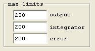
Tuning Parameters - max limits

KMotion's max limits allow several points in the
Servo Flow Diagram to be clamped, or
limited to a specified range. The limits in the flow diagram are shown as
a clamp symbol . This capability is often
useful in controlling how the system responds to extreme situations.
Maximum output limit is used to limit the maximum applied value, in counts, to the output drive. The output drive may be either one of the on-board PWM outputs or a DAC value that drives an external amplifier.
Maximum integrator limit is used to restrict the maximum value of the integrator. This effect is often used to avoid an effect referred to as integrator "wind up". Without any integrator limit, consider the case where somehow a substantial error is maintained for a significant period of time. For example turning a motor shaft by hand for several seconds. During this time the integrator would ramp up to an extremely large value. When the motor shaft was released, it would accelerate at maximum and overshoot the target by a huge amount until the integrator could ramp back down to a reasonable value. This often results in a servo slamming into a limit. The maximum integrator limit prevents this from occurring. Often the main purpose for using an integrator is to overcome static friction in order to reduce the final error to zero. This usually requires only a small fraction of total output range. In almost all cases it is of no value to allow the integrator to exceed the maximum output value.
Maximum error limits the maximum value allowed to pass through the servo compensator. The units are the same as position units. Typically, when a servo loop is operating normally, its following error is a small value. When some extreme even occurs, such as a sudden large step command, or possibly a large disturbance the error may become very large. In some cases there may be benefit to limiting the error to a reasonable value.
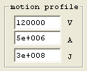
Tuning Parameters - Motion Profile

The Motion Profile parameters set the maximum allowed velocity (in position units per second), the maximum allowed acceleration (in position units per second2), and the maximum allowed jerk (in position units per second3). These parameters will be utilized for any independent (non coordinated motion) move command for the axis. The acceleration and jerk also apply to jog commands (move at continuous velocity) for the axis.
Tuning Parameters - Feed Forward

KMotion's Feed Forward may often be used to dramatically reduce the following error in a system. See the Servo Flow Diagram to see precisely how it is implemented. The idea behind feed forward is to observe the velocity and acceleration of the command signal and anticipate a required output and to apply it without waiting for an error to develop.
Most motion systems are constructed in manner where some sort of motor force is used to accelerate a mass. In these cases whenever an acceleration is required a force proportional to the acceleration will be required to achieve it. Acceleration feed forward may be used to reduce the amount that the feedback loop must correct. In fact, proper feed forward reduces the requirement on the feedback from the total force required to accelerate the mass, to only the variation in the force required to accelerate the mass.
Similarly most servo systems require some amount of force that is proportional to velocity simply to maintain a constant velocity. This might be due to viscous friction, or possibly motor back emf (electro motive force). In any case velocity feed forward may be used to reduce the demands of the feedback loop resulting in smaller following error.
The normal procedure to optimize feed forward is to select plot type - position error, and measure moves using the Move Command (Step functions should not be used as step functions are instantaneous changes in position that represent infinite velocity and acceleration).
Note that in the Servo Flow Diagram the feed forward is injected before the final IIR Filter. This allows any feed forward waveforms to be conditioned by this filter. Feed forward pulses may be relatively sharp pulses to make rapid accelerations that may often tend to disturb a mechanical resonance in the system. Usually a system with a sharp resonance will benefit from a notch filter to improve the stability and performance of the servo loop. By placing the notch filter as the last filter in the servo loop, the feed forward waveform will also pass through this filter and the result is that the feed forward will cause less excitation of the mechanism than it would otherwise..
Tuning Parameters - Dead Band

Dead band is used to apply a different gain to the region near zero than the rest of the region. Usually either zero gain or a gain much less than 1 is used within the dead band range. See the Servo Flow Diagram for the exact location of where the dead band is inserted. Dead band is a means of introducing "slop" into a system. This usually results in less accuracy and performance, but may reduce or eliminate limit cycle oscillations while resting at the target position.
The values shown (range = 0, gain = 1) are used to defeat any dead band. The chart below shows the resulting input/output for range = 2, gain = 0. The slope of the graph is always 1 outside of the specified +/- range, and the specified gain with the +/- range.

Measurement

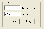
To perform a measurement and display the response, select the time duration to gather data, and the move or step size to perform, and press either the Move or Step buttons. If the axis is currently enabled, it will be disabled, all parameters from all screens will be downloaded, the axis will be enabled, the move or step will be performed while the data is gathered, the data will then be uploaded and plotted.
A Move will hold position for a short time, perform a motion of the specified amount from the current location, pause for a short time, and then a second motion back to the original location.
A Step will hold position for a short time, perform a step of the specified amount from the current location, pause for a short time, and then a second step back to the original location.
The maximum time that data may be collected is 3.5 seconds (3.5 seconds / 90µs = 38,888 data points). Note that collecting data at this rate allows zooming while still maintaining high resolution.
Axis Control

The Axis Control buttons are present to conveniently disable (Kill), Zero, or Enable an axis. If the axis becomes unstable (possible due to a gain setting too high), the Kill button may be used to disable the axis, the gain might then be reduced, and then the axis may be enabled. The Enable button downloads all parameters from all screens before enabling the axis in the same manner as the Measurement buttons described above.
Note for brushless output modes that commutate the motor based on the current position, Zeroing the position may adversely affect the commutation.
Save/Load Data

The Save/Load Data buttons allow the captured Step Plot to be saved to a text file and re-loaded at a later time. The text file format also allows the data to be imported into some other program for display or analysis. The file format consists of one line of header followed by one line of 5 comma separated values, one line for each sample. The values are:
- Sample Number
- Time, Seconds
- Command
- Position
- Output
Example of data file follows:
Sample	Time		Command	Position	Output
0	0		5	5		-0.3301919
1	9e-005		5	5		-0.3300979
2	0.00018		5	5		-0.3300258
3	0.00027		5	5		-0.3299877
4	0.00036		5	5		-0.3299999
5	0.00045		5	5		-0.3300253
6	0.00054		5	5		-0.3300359
7	0.00063		5	5		-0.3300304
8	0.00072		5	5		-0.3300199
9	0.00081		5	5		-0.3300156
10	0.0009		5	5		-0.3300157
62
.
.
.